Optimization Task
This chapter explains how to define the actual optimization task in Xoptfoil2. It assumes the previous chapters are already understood.
Table of contents
Aerodynamic Objectives
Aerodynamic objectives are defined using so-called operating points. Each operating point defines a point on the airfoil polar.
For each operating point, you define which property should be improved and how. A common objective is to minimize drag at that point.
Depending on the degrees of freedom (number of design variables) from the selected shape function, typically 3 to 10 operating points are needed for good results. Choosing the right operating points and defining the appropriate optimization target for this point is the key to successful airfoil optimization.
Defining an Operating Point
Two parameters are sufficient to define an operating point on a polar curve:
- the Re-number
- the angle of attack ‘alpha’ or alternatively the lift coefficient cl
In most cases, better results are achieved when the operating point is defined by lift coefficient cl. This is also the default mode.
For an alpha-based operating point, the optimizer may “sneak” a low drag value by reducing lift. However, alpha-based points are required when optimizing cl max, where cl itself is the quantity of interest.
To specify Reynolds numbers for operating points, convenience parameters are provided for default values. The option re_default_as_resqrtcl allows using T2 polar logic. In this case, Reynolds number is interpreted as Re*sqrt(cl).
&operating_conditions                            ! options to describe the optimization task

  re_default             = 400000                ! use this Reynolds number for operating points
  re_default_as_resqrtcl = .false.               ! interpret re number as type 2 (Re*sqrt(cl))
  mach_default           = 0.0                   ! use this Mach number for operating points

/
Once an operating point is defined on the polar, the optimization objective for this point is specified.
Min/Max Objectives
A typical objective is to minimize or maximize an aerodynamic coefficient at that operating point. The objective type is set with optimization_type. For a min/max optimization, possible values for this option are
optimization_type | Description |
|---|---|
min-drag | Minimize drag - more correctly: minimize the drag coefficient cd |
max-glide | Maximize glide ratio ‘cl/cd’. This is equivalent to ‘min_drag’ if the operating point is defined on the basis of cl |
min-sink | Minimize the sink rate cd²/cl³ |
max-lift | Maximize lift - more correctly maximize the lift coefficient cl. Only makes sense if the operating point is defined on the basis of alpha |
max-xtr | Move the laminar-turbulent transition location as far towards the trailing edge as possible. The mean value of upper and lower side is taken as the objective |
Min/max objectives should be used as sparingly as possible, as operating points usually have competing objectives and the optimization results are then no longer deterministic (see Pareto Front).
Target Objectives
Target objectives are more powerful and more versatile than min/max objectives. A target_value is specified for the operating point. If this target_value is reached during optimization, the optimizer can concentrate on the other operating points, so to speak, which leads to more reproducible results overall.
optimization_type | Description |
|---|---|
target-drag | Drag coefficient cd to be achieved for this operating point |
target-glide | Glide ratio cl/cd to be achieved for this operating point. This is equivalent to target-drag if the operating point is defined on the basis of cl. |
target-moment | Moment coefficient cm to be achieved for this operating point |
target-cp-min | Target for minimum pressure coefficient cp_min of the operating point (target_value must be negative) |
For target-drag and target-glide, target_value must be >= 0. For target-cp-min, target_value must be < 0 because cp_min is a suction coefficient.
The default behavior is that target values may also be exceeded (allow_improved_target = .true.). In rare cases, it is useful to hit a target exactly and not exceed it (allow_improved_target = .false.).
Reverse engineering
An interesting variant of optimization can be implemented with ‘Target Objectives’: Reverse engineering of an airfoil.
To do this, an existing polar curve, for example from a publication, is mapped with the help of 5-10 operating points and ‘target_drag’. The optimizer then generates the airfoil associated with this polar curve. If the operating points are well chosen, the result is an amazingly good reproduction of the original airfoil.
Flap Optimization
A special option is the definition of flaps. The optimization can then either be carried out with a fixed flap angle per operating point - or the flap angle becomes part of the optimization. In this case, each operating point with a flap angle to be optimized requires an additional ‘design variable’.
The definition of an optimization with flaps requires two sections:
- definition of the flap position and the hinge line
- specification per operating point, whether fixed angle or angle to be optimized
&operating_conditions                            ! options to describe the optimization task

  use_flap               = .false.               ! activate flap setting or optimization
  x_flap                 = 0.75                  ! chord position of flap
  y_flap                 = 0.0                   ! vertical hinge position
  y_flap_spec            = 'y/c'                 ! ... in chord unit or 'y/t' relative to height
  flap_angle_default     = 0.0                   ! default flap angle for all op points

! per operating point
  flap_angle(1)    = x                           ! flap angle (default: flap_angle_default)
  flap_optimize(1) = .false.                     ! optimize this flap angle
/
Even if flap angle is optimized, define a reasonable starting value so the initial airfoil can reach the requested operating point. If, for example, the objective is around cl=1.6 but the seed airfoil without flap reaches only cl=1.2, optimization can already fail during initialization. In this case, set an initial flap angle such as 5 degrees.
Example
Some examples of different aerodynamic objectives for operating points.
&operating_conditions                            ! some examples for operating points

  re_default       = 400000                      ! Reynolds number for all operating points
  use_flap         = .true.                      ! activate flap usage

  noppoint         = 3                           ! we define only 3 operating points

  op_point(1) = 0.2                              ! cl=0.2 as spec_cl is default
  optimization_type(1) = 'min-drag'              ! minimize cd (drag) at this point
  reynolds(1) = 300000                           ! individual Re number of this point

  op_mode(2) = 'spec-al'                         ! operating point based on alpha-value
  op_point(2) = 5.0                              ! alpha = 5.0 degrees
  optimization_type(2) = 'target-glide'          ! target is glide ratio cl/cd
  target_value(2) = 74.3                         ! objective is a glide ratio of 74.3

  op_point(3) = 1.1                              ! cl = 1.1 as spec_cl is default
  optimization_type(3) = 'target-drag'           ! target is drag cd
  target_value(3) = 0.0120                       ! target drag coefficient cd
  flap_angle(3) = 3.0                            ! set fixed flap angle of 3.0 degrees

/
Geometric Objectives
Geometric objectives work similarly to aerodynamic target objectives. They are used, for example, when the optimized airfoil should have a specific maximum thickness, or when an airfoil family should share the same maximum camber to align zero-lift behavior.
Geometric objectives compete with aerodynamic objectives and are equally weighted in determining the objective function.
Example
Some examples of geometric objectives.
&geometry_targets                                ! geometry target example
  ngeo_targets     = 2                           ! no of geometry targets

  target_type(1)   = 'thickness'                 ! objective is maximum thickness
  target_geo(1)    = 0.09                        ! target value of 9% to achieve

  target_type(2)   = 'camber'                    ! objective is maximum camber
  target_geo(2)    = 0.02                        ! target value of 2% camber to achieve
  weighting_geo(2) = 2.0                         ! higher weighting of this target
/
Objective Function
At the start of an optimization, the seed airfoil is evaluated at all operating points and each result is normalized to 1.0 using an individual scaling factor.
These individual results are then added to form an overall result, the objective function, which is normalized again to 1.0. This ensures the optimization task begins with objective-function value 1.0 for the seed airfoil.
During optimization, a better design has a smaller objective-function value. For example, a drop from 1.0 to 0.92 corresponds to an 8% improvement: (1.0 - 0.92) * 100 = 8.
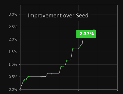
Development of the objective function during optimization, shown here as “improvement”.
Multi Objectives - Pareto Front
If results from multiple operating points are combined into one number, a known issue appears: different per-point improvements can produce the same overall result.
The (infinite) set of such equivalent trade-offs is called the Pareto front.
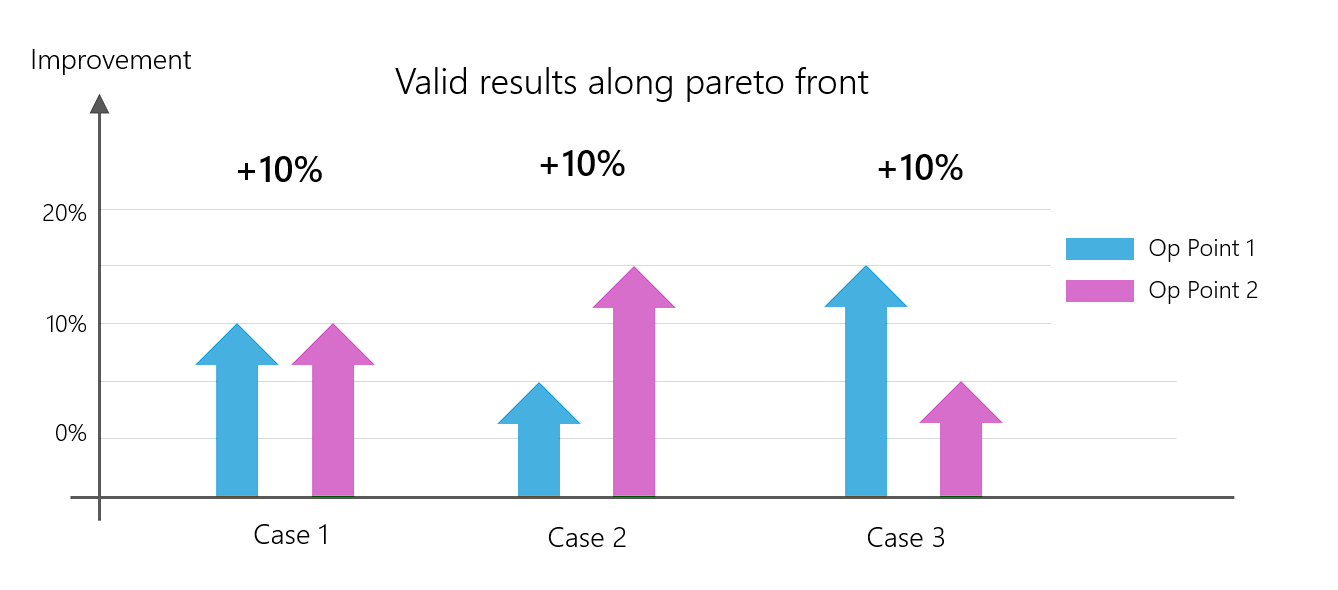
Pareto front of an optimization with two operating points. All three variants of individual-point improvement lead to the same overall result: +10%.
Which of these three results is better depends on design priorities. For example: “Result 2 is best for my use case because operating point 2 matters more than operating point 1.”
Goal Attainment
Xoptfoil2 uses goal attainment instead of dynamic weighting. Each target operating point contributes according to how far it still is from its goal.
With allow_improved_target = .true. (default), the residual is clamped to zero once a target is reached. With allow_improved_target = .false., the residual remains symmetric around the target and any deviation contributes.
This means:
- the optimizer can focus on operating points that are still unresolved,
- there is no longer a periodic dynamic reweighting step,
- target-based optimizations are easier to reproduce.
The regular weighting() parameter still exists and is used to express relative priority between operating points. It no longer serves as a dynamic corrective mechanism.
Weighting
The Pareto-front ambiguity can be reduced by weighting individual operating points. The default weighting for each operating point and each geometric objective is 1.0.
This weighting can be adjusted per operating point via weighting().
Example:
op_mode(1)   = 'spec_cl'
op_point(1)  = 0.4                             ! cl = 0.4
optimization_type(1) = 'min-drag'              ! optimize drag
weighting(1) = 2                               ! double weighting compared to default
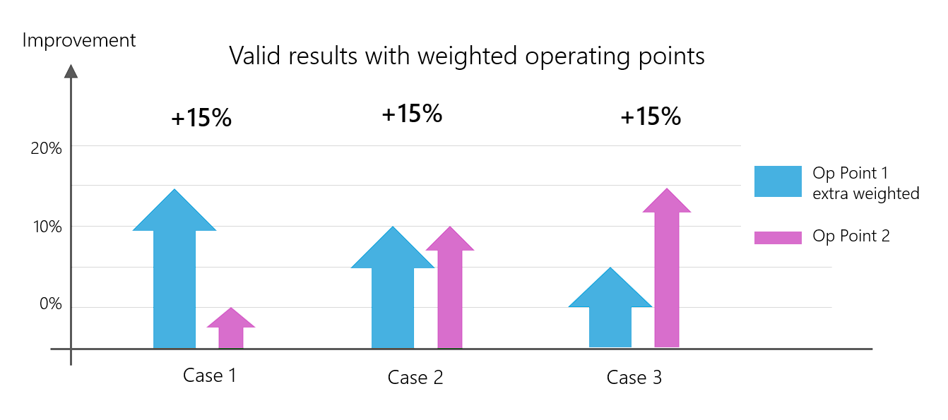
The relationship between the results can be influenced by weighting the results of the operating points differently.
Although weighting does not remove the Pareto-front issue in theory, in practice it often leads to clearer and more reproducible results.